Lab 9: Centripetal force with a motor; Lab Partner: Jamie Lopez; 10-09-2016

2) In this experiment, we will accomplish to show the relationship between angular velocity(ω) and theta(Ө) when an object rotates in centripetal motion.

3) In order to find the relationship between the angular velocity and theta, we first have to find what is rotating in centripetal motion. In this experiment, we will have a mass pulled by a string in rotation. We know that the sum of forces is equal to mass and acceleration or mass times radius times angular velocity square. Drawing a free body diagram gives a better demonstration of the external forces acting on the object. We separate the sum of forces into x and y components to where sine and cosine represents Ө into the equation. Here is a picture with a better illustration of finding the relationship between the angular velocity and theta.. Now this relationship only applies when the angular velocity remains constant over time.

4) We will be using an apparatus to find the angular velocity in two methods. Finding ω by theta by imputing it in the equation and by time for using a stop watch for every rotation the mass passes by. Here's a picture of the apparatus for a better visual.
First, we will use the formula and input Ө by solving using the Pythagorean Theorem between the height of the apparatus, height of the mass above ground, and the length of the string attached to the mass. . In this result, we notice as theta increases, the magnitude of the angular velocity and the height of the mass above the ground increases.

5) After finish recording the experiment and imputing the data and values, here are the results we find using the equations between theta and ω and theta and time.  In the second picture, the angular velocity is equal theta over time. So every time the mass rotates in full 360 rotation, that would be our marking point of how long the mass takes to rotate in one revolution. These two equations we're representing of solving ω by theta and time should equal each other. But of course, there is an uncertainty error in the time equation due to human error.

6)

7) Technically, the graph should be similar to each other of the data points. The results we got are pretty close to each other. It's off around 6%.  The x-axis is theta we measured in the experiment. The y-axis are the equations we input using theta.

8) This is the proof of the relationship between the angular velocity and theta. As the angel theta increases over time, the angular velocity increases its rate over time; assuming it remains constant.

Lab 8: Centripetal Acceleration vs angular frequency, Lab Partner: Jamie Lopez 10-03-16

2) In this lab, we will determine the relationship between centripetal acceleration and angular speed.

3) Centripetal acceleration is the rate of change of tangential velocity. The speed remains a constant magnitude but the direction changes as the object rotates. In order to prove this mathematically, we use the radius (r) from the center of the circle to the end of the circle, and define r in horizontal and vertical components. Since r will be out position of theta over time as the object rotates, we derive it until we get our acceleration which is omega square over r. Here is a picture with a better demonstration of our proof. 

4) We will prove in this lab that our theory is correct. We use an apparatus of a circular motor platform. A mass is nearly on the edge of the circular platform with a string attached to the center of the circle. In the lab we changed the radius, angular velocity, and the mass to get different results and what relationships these components give to each other.. The device that is by the center is a logger pro device to detect the force between the string and the mass and the angular velocity. Since the centripetal acceleration points towards the center of the circle, its intuitive that there is force also acting towards the center of the circle as well.

5) In each test experiment, we wrote down the values we calculated according to logger pro's devices and the settings we adjusted.. The components that are measured in the experiment are mass in grams, the radius in meters, a machine that varies different voltage readings to control the rotating motor of the circular platform, 10 revolutions as one reading, total time for 10 rotations, and the force the device read as it spanned which should be constant.

6)
We graphed three different relationships these values share in the equation. The force vs angular velocity increases as your increase the magnitude of the angular velocity. I only used for rows to graph since the mass and the radius is the same for each test result. The slope is the relationship of the mass and the radius. Here is an example. According to the data of the four rows recorded in the graph, the slope should be 0.108 kg*m and the slope the graph represents is 0.115. So our error percentage is around 7 percent. The same concept applies to the other graphs except the x-component is now the radius and mass.

8) According to our theory we represented, the lab proves our theory is accurate when we want to find the relationship between the centripetal acceleration and angular velocity. Not only does the angular velocity shares a relationship but also the radius. The mass can also share a relationship, but mathematically, the mass values end up canceling out so it's not really a necessary value.

Lab 5: Trajectories, Lab Partner: Jamie Lopez 09-19-16

2) In this lab, we will accomplish the use of understanding of projectile motion to predict the impact point of a ball on an inclined board.

3) In this experiment, we utilize our kinematic equations to predict of how far the ball will land when it leaves the edge of the table. Since the trajectory includes horizontal and vertical measurements, we will separate them to get our results. Here are the two experiments we tested to find the total distance the ball travels when it leaves the edge of the table. 

4) The first picture represents the first experiment to solve the total distance when it leaves the edge of the table. The second and fourth pictures represents the second experiment. The third picture is a carbon sheet of paper. We use the carbon paper to make the landing of the ball. We repeat the process of both experiment twice to make sure we get the same results. Our measurements from the ball's landing to the edge of the table is off by 1.5 cm since the area of the ball's landing wasn't always exactly on the same landing point.

5)

6)Since we didn't use a logger pro device to determine a graph, here is an example of the ball's position and velocity the moment it leaves the edge of the table.


7) The pictures in number 5 are the calculations to determine the distance the ball leaves the table. Since we did have an uncertainty by 1.5 cm, our results still gives us an uncertainty around 1 cm. But our theory lets us predict correctly what we wanted to find by using the kinematic equations for projectile motion.

Lab 7: Modeling Friction Forces, lab partner: Jamie Lopez, Date: 09-23-16

2) In this experiment, we are going to derive different experiments that include friction.

3) There are five experiments we are going to work on. They are static friction, kinetic friction, static friction from a sloped surface, kinetic friction from sliding a block down an incline, and predicting the acceleration of a two massed system. We want to calculate the coefficient of static and kinetic friction by using the logger pro devices and using the formulas of what we learned so far.

4) In the static friction experiment, we used a smooth long board attached to a pully. We put a block on top of the board and a mass unknown amount hanging. Once the block moves forward we determined our static friction. For kinetic friction, we attached a string to a device to detect the Newton measurement as the object is pulled forward. Next, we elevated the board and determine its angle and find when the block slides as the slope increases for the static friction. Then, we determined the kinetic friction as it slides down the board and find the coefficient. Lastly, we predict the acceleration of a two mass system.

5)

7) In the first page, we wrote down the data of the mass we calculated in our experiment. We solved to find the coefficient for static friction and the kinetic friction according to the equation. On the next page, we did the same procedure but analyzed to see if the coefficient of static and kinetic friction would be any different if the object moving was on an elevated surface. The last page we conducted an experiment to find the acceleration of the 2 masses on a pulley. We solved for the acceleration according to the equation on the page and used the logger pro device to see if our calculations were accurate. Our calculations were off by 0.09 meters per second squared which is not that far off.

8) According to our calculations, our results came out pretty accurate. We followed the equations of Newton's Laws of Forces and repeated our experiment to make sure we would get the same results more than once. The hardest part in the experiment was finding the static coefficient of friction because once we deducted a small amount of mass the instant the object moved, our uncertainty was off by 5 grams of mass.

07-Sept-16: Non-Constant Acceleration

1) Rafael Vera
Lab Partner: Jamie Lopez

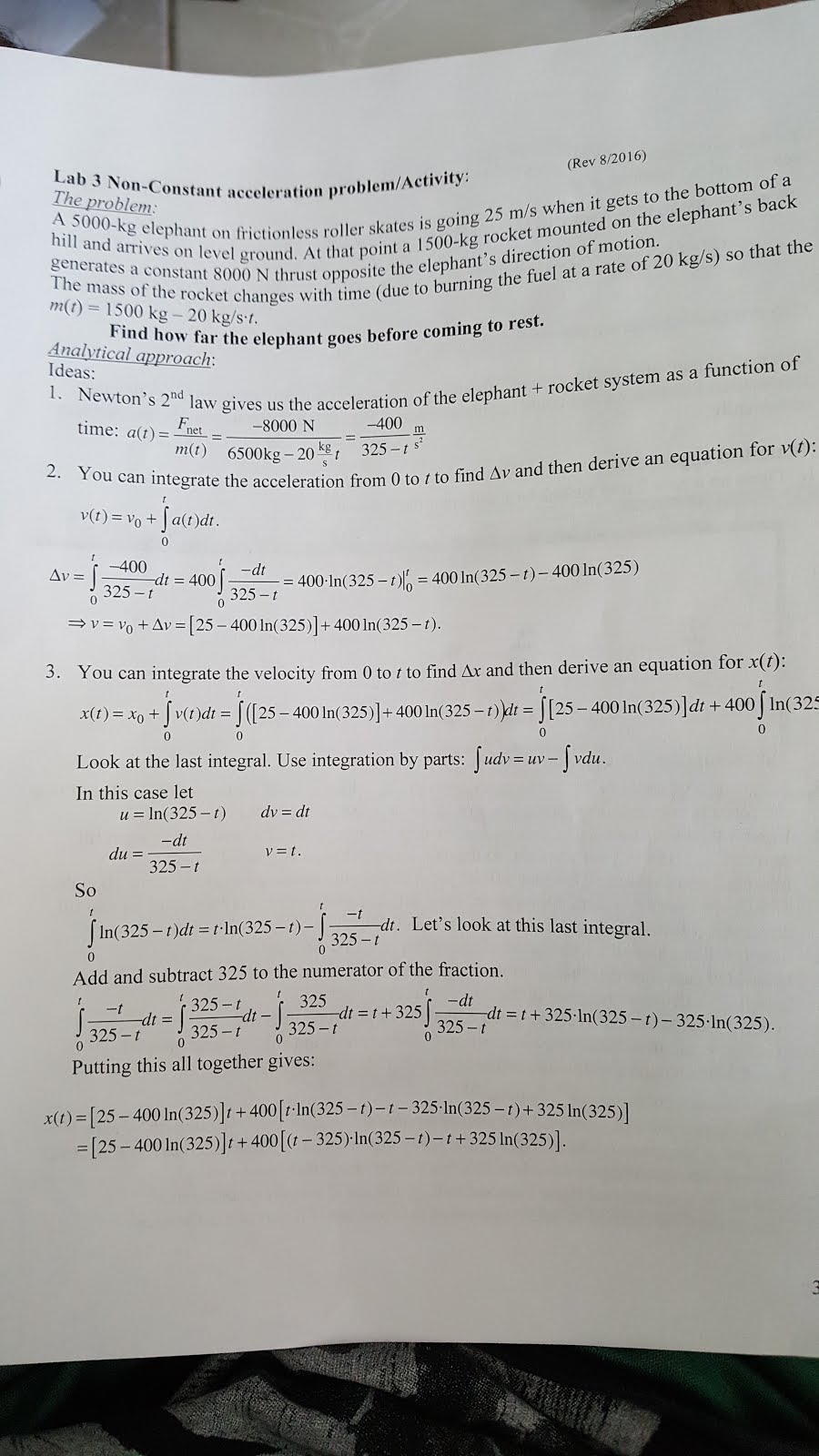
2) In this lab, we are experimenting to convert equations from integrating to inputting them on Excel to visually see the computer's calculation.

3) In the real world applications, it is more than just entering equations and memorization. We have to understand the relations why we use the formulas and the equations to find our measurements. There's a basic understanding when applications introduces kinematic problems because people experiment it everyday. Using calculus integration can be easy sometimes to find what we want; however, with complicating equations it can be time consuming and overall a big mess. Fortunately with technology, we have a method that can do the dirty work for us.

4) The application of Windows Excel can input the work for us as long we have the values. Windows Excel is an electronic spreadsheet that features calculations, graphing tools, pivot tables, and etc. by entering data and formulas in the cell columns.

5)
This is an example problem given in lab. With the given values, we entered the formulas in the cells to get the answer in the columns; for example to find the average velocity. We separate each cell column in categories to find our answers it calculates over time. Just like in calculus integration when time difference approaches zero, we can modify the time difference in our data sheet as it approaches to zero.

6) For the Position-Time Graph, the Y-axis is in meters and X-axis is in seconds. For the Velocity-Time graph, the Y-axis is in meters per second and X-axis is in seconds.

7) Putting our data into a graph can make us visually understand what is happening; for example, the rate of how fast the elephant is slowing down. The position-time graph slightly shows a slope since the entry in the data table is only 5 seconds within 100 cells.

8) The data spread sheet computes our calculations as we input formulas in the cells. By using the example of the elephant, we can compare if both methods come out as the same.

05-Sept-2016: Free Fall Lab with Mean Deviation

1) Rafael Vera
Lab Partner: Jamie Lopez

2) In this experiment, we learn about propagated uncertainty and relate it on an example: finding the acceleration of gravity on Earth.

3) Measurements aren't all accurate as we count them on a tally mark. Our estimate can be off greatly or close enough. One way of calculating to have your lab results to be sufficient to your expected results is the standard deviation of the mean. The standard deviation of the mean is a way of describing the spread of the data. It calculates the average of how close of the combined results taken by different tests to the expected conclusion; or in this case your uncertainty.

4) The experiment we choose is a free fall apparatus. The apparatus is a sturdy column, about 1.5 meter falling distance, for accurate reading. When the free fall body, held at the top by an electromagnet, is released, its fall is precisely recorded by a spark generator. The marks that are made on the sheet of tape is what we count as the displacement for every mark noted. We use a meter stick to write down the measurement. This is where the uncertainty follows in. We used our estimated guess of where the mark is and compare other grouped by using the standard deviation of the mean.

5)
This is the data we recorded from the meter stick. Each data information is the distance from the point to the 0 mark of the stick.

6)
The graph on top represents the Mid-interval speed vs. Mid-interval time. The units in the y-axis is in meters per second and the x-axis is in seconds. The interval in the x-axis is measured 1/60th of a second. The graph on the bottom represents the Distance vs. Time. The time interval in the x-axis is also measured 1/60th of a second.

After finishing our data points, we compared to the other groups in class. These are the results given.

7) So for the data we recorded, we plugged them in the formula in Excel and convert it in a graph which gave us a slope to what we expected. The distance graph gradually changes over time as the object falls. We derived the Distance vs Time graph and got the Velocity vs Time graph. It's a constant slope as the object falls over time. Our data is a little off as you can tell the square dots we inputted are not very specific in a straight slope. This is an ideal visual of what we determine of propagated uncertainty. For the data on the bottom, we used the standard deviation of the mean and the results shows us how far off each group is by the mean. Unfortunately my readings are the most far off results to the expected results.

8) Our experiment shows of how much error we can be off when it comes to measuring. We followed up the results we tried hoping for to get the expected results. If the markings on the tape were more accurate and the measuring tool were more precise, our error would have been much less than what our answer was.

29-Aug-2016: Finding a relationship between mass and period for an inertial balance

1) Name: Rafael Vera

Lab Partner: Jamie Lopez

2) In this lab, we will prove that mass is a measurement of constant inertia, even with a disturbance force of gravity affecting it. 

3) In order to prove that mass is a physical property that remains constant, we must use a device to measure its oscillation. if it remains a constant period, then our theory is correct. We also must look for an equation of how mass relates when its resistant to an acceleration force.

4) 
We used a device called the Inertial Balance to measure the inertial mass by comparing objects' resistance to changes in their motion. We used a c-clamp to secure the inertal balance on the tabletop and put a thin piece of tape on the end of the inertal balance so when we plug in a photogate device sensor to a laptop, it will calculate when the masking tape passed the sensor and returned. Once the tape returns, it will be known as one period or oscillation.

5) These are the results by using logger pro of the data table. we used increments of 100 g mass to find an average period when the apparatus commences its' results.

These two graphs explain the Max and Min rate as the object oscillates in the duration time of 7 seconds. The slope explains the relationship between the period and the mass.

6) The next similar experiment we did was to put a random object on the apparatus and find its mass by the following formula: 
Here are the two objects we used in the lab to find its mass:
Calculator




Phone

7) Two objects were chosen to be tested so there would be same results on our theory. As the two objects are oscillating on the Inertial Balance apparatus, they both give the same result of conserved mass. Both masses do not change over time as they're being accelerated by force. The slope is what shows that both masses do not change.

8) In essence, this experiment proves our theory about inertial mass. Since we cannnot measure the quantity of mass on a weight scale due to gravitational force, we plug in the relationship of period and mass equation and gives us a more accurate reading.